The worksheet functionality in the Vectorworks program complements its drawing functionality, making it a complete package for your work process. From the information present in the file, you can create worksheets to track data, create cost and material lists, perform calculations, and more. Worksheets are integrated within the Vectorworks file, which eliminates the need for a separate program and reduces the number of files per project.
Worksheets include both database and spreadsheet functionality. Data can be obtained from the drawing, and then calculations can be performed on that data.
Worksheets can be imported and exported, which allows data to be shared between worksheets, files, and other spreadsheet programs. A worksheet can also be added to a drawing and printed.
To get a quick overview of worksheet features, see “Worksheet Tutorial: Creating a Wall Schedule” on page 1357.
~~~~~~~~~~~~~~~~~~~~~~~~~
For complex drawings, it is best to create separate worksheets for each task rather than one large worksheet. Worksheets can be linked to share data, formulas, and calculations.
Worksheets can be created in several ways:
• Use the Create Report command to select worksheet data from the information associated with the objects in the drawing. See “Creating Reports” on page 1312.
• Use the Resource Browser to create a blank worksheet, and then add the desired information to it. See “Creating a Blank Worksheet” on page 1313.
• Import worksheets from other Vectorworks files or from other spreadsheet programs. See “Importing Worksheets” on page 1354.
• If Vectorworks Design Series is installed, preformatted records and schedules such as room finishes, plant lists, and lighting instruments can be added to the drawing. See “Creating Schedules” on page 1858 and “Creating Schedules Automatically” on page 1314.
Once created, a worksheet is saved with the file and is listed in the Resource Browser. It can also be accessed by selecting Window > Worksheets.
If the same objects are typically used in your drawings, you can create a template file with a worksheet that serves as a “master price list” listing all the objects and their costs. Then, to create materials lists and cost estimates for a new design, simply import the worksheet into the new drawing file.
The Create Report command allows you to select data that is attached to objects in a drawing (such as manufacturer, size, and price) and create a worksheet from it. The command can either create a new worksheet or append database rows to an existing worksheet. For more information about how to attach data to objects, see “Registros” on page 257.
To create a report from objects in a drawing:
1. Select the Create Report command from the appropriate menu:
• Fundamentals, Architect, Landmark: Tools > Reports > Create Report
• Spotlight: Spotlight > Reports > Create Report
The Create Report dialog box opens. Specify the report criteria. Items in the Worksheet Columns list are listed in the order in which they will appear in the worksheet; to change the order, click in the # column and drag the item to the desired position in the list.
Click to show/hide the parameters.
2. Click Options to specify additional report criteria.
The Create Report Options dialog box opens.
Click to show/hide the parameters.
3. Specify the options for creating the report, and click OK to return to the Create Report dialog box.
4. Click OK to create the worksheet.
The worksheet opens automatically. The top row of the worksheet contains a title for each column selected. Next is a database header row (indicated by a diamond next to the row number) that contains sub-row totals for each column. Beneath the header row are sub-rows for each object or symbol in the drawing that matches the report criteria.
5. To add more data to the worksheet, repeat steps 1 through 4 and select the Append to existing worksheet option.
6. Once all the data is added, edit the worksheet as needed. For example, add rows or columns, change the text format, or add color. To hide the database header rows, toggle the Database Headers setting on the Worksheet menu.
Click here for a video tip on this topic (Internet connection required).
~~~~~~~~~~~~~~~~~~~~~~~~~
Instead of using the Create Report command, you can create a blank worksheet and add data to it manually. This gives you more control over the contents and format of the worksheet.
To create a blank worksheet:
1. Select Window > Palettes > Resource Browser.
2. Select Resources > New Resource to display the list of new resource types.
3. Select Worksheet.
The Create Worksheet dialog box opens.
Click to show/hide the parameters.
4. Specify the basic worksheet parameters and click OK.
A new worksheet window opens.
5. At this point, all rows contain spreadsheet cells, and they are all undefined. Define the contents of each row and cell as needed:
• To add simple text, numbers, or formulas to the worksheet, see “Entering Data in Spreadsheet Cells” on page 1329.
• To list data that is associated with objects in the drawing, change a spreadsheet row into a database row, and specify which objects to include in the list. A sub-row displays for each object that matches the criteria defined in the database header row. Then specify which information to display in the columns for each row; these can be fields from the object’s data record, as well as text, numbers, or formulas. See “Entering Data in Database Rows” on page 1335.
• To add images to either spreadsheet or database rows, see “Inserting Images in Worksheets” on page 1339 (Vectorworks Design Series required).
~~~~~~~~~~~~~~~~~~~~~~~~~
 Creating
Schedules Automatically
Creating
Schedules AutomaticallyThe Vectorworks Landmark and Spotlight products include a Choose Schedule command with preformatted schedules that are generated automatically. The Vectorworks Architect product includes preformatted, customizable records and schedules as described in “Records and Schedules” on page 1853. The schedules can be created any time; as objects are added to the drawing, recalculate the worksheet to update the results.
The preformatted schedules are from the default content included with the Vectorworks Design Series products in the [Vectorworks]\ Libraries\Defaults\Reports~Schedules folder (see “Resource Libraries” on page 215).
The default schedules for Vectorworks Landmark include plant lists, irrigation plans, and existing tree reports, with or without images. Plants to be included in the Plant List worksheets must have On Plant List selected in the Plant Settings dialog box or the Object Info palette.
A formatted worksheet can be saved as a custom schedule to be used again; export the worksheet resource (renamed with a custom name) to a file in the Reports~Schedules folder in your user folder. Your customized worksheet becomes available for selection in the Choose Schedule dialog box. For information about exporting resources, see “Exporting Custom Resources” on page 230.
Another way to create a schedule is to select the Create Report command. List the objects with the relevant record, such as the Existing Tree record, and then select the desired columns to include in the report. See “Creating Reports” on page 1312 for more information.
To add a schedule:
1. Select a command from the appropriate menu:
• Landmark: Tools > Reports > Choose Schedule
• Spotlight: Spotlight > Reports > Choose Schedule
• Architect: Tools > Reports > VA Create Schedule
The Choose Schedule dialog box (for Landmark and Spotlight) or Create Schedule dialog box (for Architect) opens. Select one of the worksheets to create; select Place worksheet on drawing to add the worksheet to the drawing area.
2. Click OK to create the selected worksheet.
If the selected schedule already exists in the file, a warning dialog box opens. Select whether to replace or rename the new schedule (some schedules also have a recalculate option), and click OK.
3. If the worksheet is to be placed on the drawing, click to indicate the position of the top left corner of the worksheet.
The worksheet, populated with specific information from the current drawing, is automatically created.
~~~~~~~~~~~~~~~~~~~~~~~~~
Worksheets can obtain data from the drawing based on specified criteria, and then list the data and allow calculations to be performed on the data.
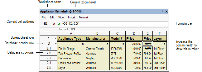
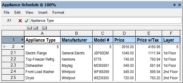
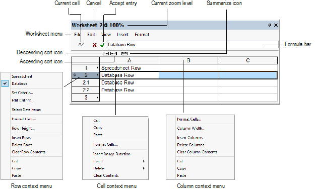
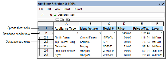
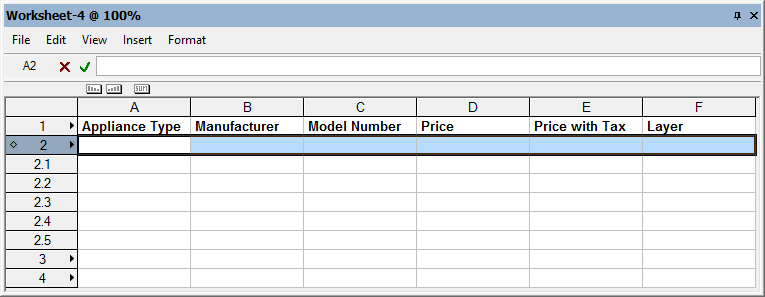
Worksheets can have two types of rows: spreadsheet and database. The cells in a spreadsheet row contain constants (text or numbers), or formulas. Database rows consist of a header row and sub-rows, and they show data that are associated with specific drawing objects. The database header row is marked with a diamond shape next to the row number. Set selection criteria for this row, and a sub-row is created for each object that meets the criteria. In this example, the database header row 2 is set to list each object in the drawing that has an “appliance record” attached to it. The sub-rows 2.1 through 2.5 represent the five objects in the drawing that meet this criteria.
Rows are numbered sequentially starting with 1, and columns are labeled alphabetically starting with A. Database sub-rows are numbered with the database header row’s number, followed by a decimal and sequential numbers (header row 2 has sub-rows 2.1, 2.2, 2.3, and so on). The cell’s column letter and row number indicate the spreadsheet cell address, as in A4 or D2 (database sub-rows display a blank address).
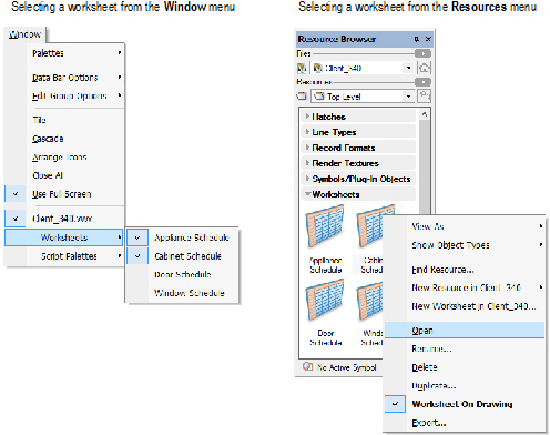
When worksheets exist in an open file, the Window > Worksheets command becomes available. All the worksheets present in the indicated file are listed. Worksheets with a check mark are currently open. To open a worksheet, select it from this menu, or select the worksheet from the Resource Browser and then select Resources > Open.
A worksheet opens in a separate window, which can be resized, moved, and closed. The worksheet window contains its own menu and context menus.
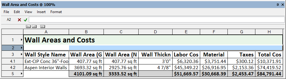
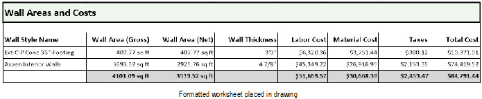
Because an open worksheet is in a separate window, it is not printed with the drawing. To include a worksheet as part of a drawing, select the worksheet in the Resource Browser and click Resources > Worksheet on Drawing. When the worksheet is open, the worksheet on the drawing displays as an “X.” When the worksheet is closed, the updated worksheet displays on the drawing. Double-click the worksheet from the drawing to open it. See “Worksheets as Graphic Objects” on page 1356.
Use the Format Cells command to format individual rows, columns, and even cells of the worksheet as needed. The format is retained when the worksheet is included on the drawing. Alternatively, with the worksheet window closed, select the worksheet object on the drawing, and use the Attributes palette to modify the fill, pen, and line thickness attributes for the entire object.
~~~~~~~~~~~~~~~~~~~~~~~~~
The contents of cells can be edited, and the rows and columns can be resized, moved, cut, copied, and pasted.
The following table describes the keys used to move around in the worksheet.
Keys |
Description |
|---|---|
Arrow (Up, Down, Right, Left) |
Moves by one cell in the direction indicated |
Tab |
Moves right by one cell |
Enter |
Moves down by one cell |
Shift+Tab |
Moves left by one cell |
Shift+Enter |
Moves up by one cell |
If more than one cell is selected, movement is restricted to the selected cells only.
Selected cells are surrounded with a black outline. When multiple cells are selected, the active cell is white, and the remaining selected cells are highlighted in blue.
Selection |
Action |
|---|---|
A single cell |
Click on the cell |
A range of cells |
Click-drag across a range of cells to select them, or click in one corner and Shift-click in the opposite corner |
An entire column or row |
Click the column letter or row number; to select multiple rows or columns, click-drag across the column letters or row numbers, or click the first column letter or row number, and then Shift-click the last column letter or row number in the desired range |
Non-contiguous cells, rows, or columns |
Press and hold the Ctrl (Windows) or Command (Mac) key and then click on each cell, row, or column to select |
The entire worksheet |
Click the empty box directly above the row number boxes |
When a cell is selected, the display of the Formula bar indicates whether the contents of the cell can be edited.
Formula Bar Display |
Explanation |
|---|---|
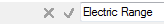
The cell address displays, and the red X and green check mark are active |
The cell is in a spreadsheet row or database header row. Type directly in the Formula bar to enter text, numbers, or a formula. To accept the edits and change the cell contents, click the green check mark. To cancel the edits, click the red X. |
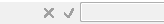
No cell address displays; the current cell value is not editable |
In database sub-rows, the results of calculations cannot be edited. In addition, object attribute information, such as the class the object belongs to, cannot be edited in the worksheet. |
No cell address displays; the current cell value is editable (Vectorworks Design Series required) |
In database sub-rows, if Vectorworks Design Series products are installed, information that comes from the object’s data record can be edited in the Formula bar, and the object’s record is updated automatically. For example, the price data for a sub-row object could be updated. To accept the edits and change both the worksheet and record, click the green check mark. |
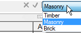
No cell address displays; a list of the values that are available for the current cell displays (Vectorworks Design Series required) |
In database sub-rows, if Vectorworks Design Series products are installed, some fields that come from the object’s data record can be edited, but they only allow certain pre-defined values. For example, the sill style for a window sub-row object could be changed in the Formula bar. Select the new value from the list to change both the worksheet and record. |
Neither a cell address nor a cell value displays
|
In database sub-rows, if the Vectorworks Architect or Vectorworks Landmark product is not installed, information that comes from the object’s data record cannot be edited in the worksheet. To edit a value that displays in a sub-row, right-click (Windows) or Ctrl-click (Mac) the number of the row that is associated with the item in the drawing, and select the Select Item command from the context menu. Then use the Data tab of the Object Info palette to edit the object data as needed. |
To adjust column width or row height, drag the divider bar between the column letters or row numbers. If you select multiple rows or columns before you drag the bar, all rows or columns are adjusted to the same size.
Alternatively, select the Column Width command from either the Format menu or the column context menu (see “Column Width” on page 1322). Adjust the row height with the Row Height command from either the Format menu or the row context menu (see “Row Height” on page 1322).
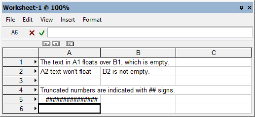
Text that is longer than the width of a cell “floats” over empty adjacent cells. Numbers that exceed the cell width are displayed with # characters. Alternatively, text can be set to wrap (see “Formatting Worksheet Cells” on page 1326).
To hide a row or column, set the Column Width or Row Height to 0. To display the column or row again, position the cursor over the column letter or row number adjacent to the hidden column or row. When the cursor changes to a double bar resize cursor, click-drag the bar to resize the column or row.
The standard shortcut keys for Cut and Paste can be used for worksheet editing. The same value or formula can be copied and pasted to a range of cells.
To copy cell contents to a cell or range of cells:
1. Select the cell with the information to repeat, and then press Ctrl+C (Windows) or Command+C (Mac) to copy the cell.
Alternatively, select the Copy command from either the Edit menu or the appropriate context menu (see “Copy” on page 1321).
2. Select the destination cell(s) for the information, and then press Ctrl+V (Windows) or Command+V (Mac) to paste. The formula or value is repeated in each of the selected cells.
Alternatively, select the Paste command from either the Edit menu or the appropriate context menu (see “Paste” on page 1321).
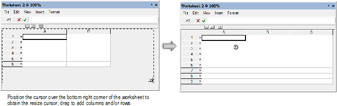
From the Insert menu, you can insert rows and columns (see “Worksheet Commands” on page 1320). An empty row is added above the current row, or an empty column is added to the left of the current column. Another option is to position the cursor at the bottom right corner of the worksheet to activate a special resize cursor; drag as needed to add rows and columns to the bottom and right side of the worksheet.
Use the drag and drop method to move contiguous rows and columns or to move a copy of contiguous rows and columns.
To move a copy of rows or columns:
1. Click the column letter or row number to select a column or row (click-drag across the letters or numbers to select multiple columns or rows).
2. Press and hold Ctrl (Windows) or Option (Mac) and move the cursor to the edge of the selected rows or columns. When the cursor changes to a copy cursor to indicate that moving a copy is permitted, drag the selection to the desired location in the worksheet.
To move rows or columns:
1. Click the column letter or row number to select a column or row (click-drag across the letters or numbers to select multiple columns or rows).
2. Move the cursor to the edge of the selected rows or columns. When the cursor changes to a move cursor to indicate that moving the rows or columns is permitted, drag the selection to the desired location in the worksheet.
~~~~~~~~~~~~~~~~~~~~~~~~~
Various command menus are available in the worksheet window, as well as sorting functions. The main worksheet menu is at the top of the window. Right-click (Windows) or Ctrl-click (Mac) on a specific worksheet row or cell to open a context menu. To sort the sub-rows associated with a database header row, click and drag a sort icon to the column header cell.
~~~~~~~~~~~~~~~~~~~~~~~~~
The main Worksheet menu commands are described in the following table.
Worksheet Command |
Description |
|---|---|
File menu |
|
Recalculate |
Recalculates all formulas in all worksheets, whether open or closed. This function can also be accessed from the context menu of the worksheet image (on the drawing): right-click (Windows) or Ctrl-click (Mac) on the worksheet, and select Recalculate. |
Opens the Worksheet Preferences dialog box. Header and Footer text fields and the Margin settings apply to printed worksheets only. Select Show Grid to display the worksheet gridlines. Select Show Tabs to print worksheet column and row headers. Select Auto-recalc to recalculate all worksheet arithmetic functions when cells are edited. Click Font to specify the worksheet default font and size. |
|
Printer Setup |
Opens the Printer Setup dialog box. This is the same as the standard Printer Setup dialog box; however, it only affects the printer information for the worksheet. |
Opens the Print dialog box, to print the current worksheet; this is the only way to print a worksheet unless the worksheet is included as a part of the drawing |
|
Edit menu |
|
Undo |
Undoes the last worksheet change; execute the command multiple times to undo multiple actions |
Redo |
Reverses the last Undo command; execute the command multiple times to redo multiple undo actions |
Cut |
Removes the contents of selected cells, temporarily storing the contents in the clipboard |
Copies the contents of selected cells to the clipboard, where they are temporarily stored; the original contents remain in the worksheet |
|
Places cell contents stored in the clipboard into the current cell or range of cells |
|
Clear Contents |
Deletes the contents of the selected cells |
Delete Rows |
Deletes the selected row(s) from the worksheet. Use caution when deleting a row. Deleting cells that are part of a formula may change the values returned by the formula. |
Delete Columns |
Deletes the selected column(s) from the worksheet. Use caution when deleting a column. Deleting cells that are part of a formula may change the values returned by the formula. |
View menu |
|
Database Headers |
Toggles between displaying and hiding all worksheet database header rows |
Grid Lines |
Toggles between displaying and hiding grid lines between the rows and columns of the worksheet, in both the worksheet window and the worksheet image (on the drawing) |
Zoom |
Increases or decreases the zoom percentage by preset levels from 50% to 300%; the current zoom level displays in the worksheet title bar. Select a zoom level from the Worksheet menu, or roll the mouse wheel while holding Ctrl (Windows) or Option (Mac) to increase or decrease the zoom level by increments of 10% (regardless of the number of lines you assigned the mouse to scroll in the mouse setup). This feature will not work properly if standard scrolling is disabled in the mouse setup. For example, if the mouse’s scrolling size is set to “none,” mouse zooming in the Vectorworks program is disabled. (The specific settings required for this feature depend on the type of mouse being used.) |
Insert menu |
|
Rows |
Adds rows to the worksheet, above the selected row(s). The number inserted depends on how many rows in the worksheet are highlighted at the time the command is selected. Use caution when inserting rows. Depending on the type of cell references used in formulas, inserting rows could change the values returned by a formula. |
Columns |
Adds columns to the worksheet, to the left of the selected column(s). The number inserted depends on how many columns in the worksheet are highlighted at the time the command is selected. Use caution when inserting columns. Depending on the type of cell references used in formulas, inserting columns could change the values returned by a formula. |
Function |
Opens the Select Function dialog box; select a function to be inserted in the formula (see “Entering Formulas in Worksheet Cells” on page 1331) |
Criteria |
Opens the Criteria dialog box; select search criteria to insert in a formula |
Image Function (Vectorworks Design Series required) |
Inserts the image function in the formula for the current cell |
Format menu |
|
Cells |
Opens the Format Cells dialog box, for setting the format and appearance of selected cells |
Opens the Column Width dialog box. Set the width value of selected cells in the specified units. Click Standard Width to use the default width. The width of multiple selected columns can be adjusted at one time. |
|
Opens the Row Height dialog box; set the row height to automatically fit the selected cell contents, or set a specific row height in the specified units. The height of multiple selected rows can be adjusted at one time. |
~~~~~~~~~~~~~~~~~~~~~~~~~
To access the commands available for a specific worksheet cell, right-click (Windows) or Ctrl-click (Mac) on the cell.
Menu Item |
Description |
|---|---|
Cut |
Removes the contents of selected cells, temporarily storing the contents in the clipboard |
Copy |
Copies the contents of selected cells to the clipboard, where they are temporarily stored; the original contents remain in the worksheet |
Paste |
Places cell contents stored in the clipboard into the current cell or range of cells |
Format Cells |
Opens the Format Cells dialog box, for setting the format and appearance of selected cells |
Insert Image Function (Vectorworks Design Series required) |
Inserts the image function in the formula for the current cell |
Insert |
Adds rows or columns to the worksheet. The number inserted depends on how many rows or columns in the worksheet are highlighted at the time the command is selected. Select Insert > Rows to insert above the selected row(s). Select Insert > Columns to insert to the left of the selected column(s). Use caution when inserting rows or columns. Depending on the type of cell references used in formulas, inserting rows or columns could change the values returned by a formula. |
Delete |
Deletes rows or columns from the worksheet. Select one or more rows or columns and select Delete > Rows or Delete > Columns. Use caution when deleting a row or column. Deleting cells that are part of a formula may change the values returned by the formula. Select Edit > Undo to undo the action. |
Clear Contents |
Deletes the contents of the selected cells |
Pick Value from List |
If the cell is in a database sub-row, and the column lists a field that only allows certain pre-defined values, use this option to edit the object’s data. For example, you might want to change the sill style for several window objects from the window schedule. Select the Sill cells for the objects to be changed, and right-click (Windows) or Ctrl-click (Mac). Select a different sill type from the list of options to change both the worksheet and the objects’ data records. |
~~~~~~~~~~~~~~~~~~~~~~~~~
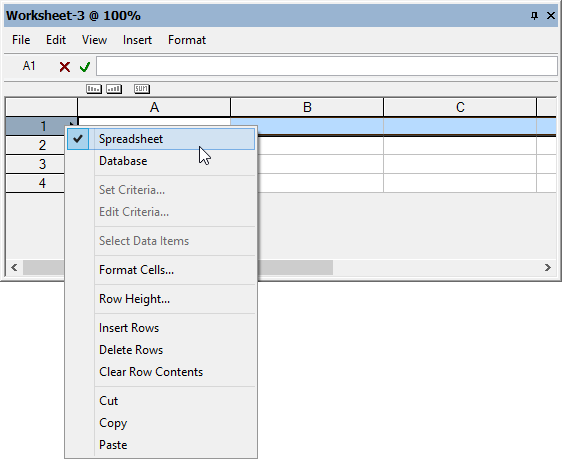
To access the commands available for a specific worksheet spreadsheet or database header row, right-click (Windows) or Ctrl-click (Mac) while on the row number. These commands do not apply to database sub-rows.
Menu Item |
Description |
|---|---|
Spreadsheet |
Converts a database header row into a row of spreadsheet cells. This deletes all sub-rows and the information contained within them. Any formulas that were defined in the columns of the header row remain intact. This command has no effect on spreadsheet cells. |
Database |
Converts a row of spreadsheet cells into a database header row and opens the Criteria dialog box. This command has no effect on database rows. |
Set Criteria |
Opens the Criteria dialog box for setting the criteria that is used to generate the database sub-rows. Available only when a database header row is clicked. |
Edit Criteria |
Opens the Criteria dialog box for editing the criteria that is used to generate the database sub-rows. Available only when a database header row is clicked. |
Select Data Items |
Selects all objects on the drawing that meet the criteria for the database row. Available only when a database header row is clicked. |
Format Cells |
Opens the Format Cells dialog box, for setting the format and appearance of selected cells |
Row Height |
Opens the Row Height dialog box; set the row height to automatically fit the selected cell contents, or set a specific row height in the specified units. The height of multiple selected rows can be adjusted at one time. |
Insert Rows |
Adds rows to the worksheet, above the selected row(s). The number inserted depends on how many rows in the worksheet are highlighted at the time the command is selected. Use caution when inserting rows. Depending on the type of cell references used in formulas, inserting rows could change the values returned by a formula. |
Delete Rows |
Deletes the selected row(s) from the worksheet. Use caution when deleting a row. Deleting cells that are part of a formula may change the values returned by the formula. |
Clear Row Contents |
Deletes the contents of the selected cells |
Cut |
Removes the contents of selected cells, temporarily storing the contents in the clipboard |
Copy |
Copies the contents of selected cells to the clipboard, where they are temporarily stored; the original contents remain in the worksheet |
Paste |
Places cell contents stored in the clipboard into the current cell or range of cells |
While on a database sub-row, right-click (Windows) or Ctrl-click (Mac) and select the Select Item command from the context menu. Use this command to select an individual database object in the drawing; the view changes to display the selected object (see “Importing Worksheets” on page 1354). The command is unavailable if the sub-row is summarized (see “Database Row Sort and Summary Functions” on page 1325).
~~~~~~~~~~~~~~~~~~~~~~~~~
To access the commands available for a specific worksheet column, right-click (Windows) or Ctrl-click (Mac) while on the column letter.
Menu Item |
Description |
|---|---|
Format Cells |
Opens the Format Cells dialog box, for setting the format and appearance of selected cells |
Column Width |
Opens the Column Width dialog box. Set the width value of selected cells in the specified units. Click Standard Width to use the default width. The width of multiple selected columns can be adjusted at one time. |
Insert Columns |
Adds columns to the worksheet, left of the selected column. The number inserted depends on how many columns in the worksheet are highlighted at the time the command is selected. Use caution when inserting columns. Depending on the type of cell references used in formulas, inserting columns could change the values returned by a formula. |
Delete Columns |
Deletes the selected columns from the worksheet. Use caution when deleting a column. Deleting cells that are part of a formula may change the values returned by the formula. |
Clear Column Contents |
Deletes the contents of the selected cells |
Cut |
Removes the contents of selected cells, temporarily storing the contents in the clipboard |
Copy |
Copies the contents of selected cells to the clipboard, where they are temporarily stored; the original contents remain in the worksheet |
Paste |
Places cell contents stored in the clipboard into the current cell or range of cells |
~~~~~~~~~~~~~~~~~~~~~~~~~
The group of sub-rows associated with a header row can be sorted and summarized in different ways. These functions can be set independently for each database header row in a worksheet.
The sort and summary functions cannot be used on a header cell for an image column (Vectorworks Design Series required).
To sort or summarize a group of database sub-rows:
1. If the database header rows are not displayed, select View > Database Headers from the Worksheet menu.
2. Select the header row of the group of sub-rows to sort or summarize; the header row has a diamond next to its number.
The three icons above the left end of the column header cells become available.
Icon Item |
Description |
Descending Sort
|
Sorts the database sub-rows in descending order, according to the contents of this column |
|
|
Sorts the database sub-rows in ascending order, according to the contents of this column |
Summarize
|
Summarizes the database sub-rows according to the contents of this column. Sub-rows that have identical items in this column are grouped together in a single row. If a column contains data from a numeric field, the summarized column contains a sum of the values for all objects that are grouped on the row. This may be appropriate for some columns, but not others. For example, you might have a window schedule that sorts and summarizes the data by the Window ID column. You would want the Quantity column to show the sum of all windows with a particular ID, but you would want the Window Height column to show the height of a single window with that ID (not the height of all windows combined). Add an additional summary operator to the Window Height column to show the correct numeric data. |
3. Click and drag an icon to the column header cell to be used for the sort or summary. A new icon displays next to the column heading letter. For an ascending or descending sort, a number in the icon indicates the sort precedence for that column.
4. Apply additional sort or summary icons as needed. In each group of sub-rows, up to 20 columns can have either an Ascending or Descending Sort icon, and any number of columns can have a Summarize icon. The Summarize icon can be used on a column by itself, or in conjunction with one of the sort icons.
5. To remove a sort or summary, click and drag the icon away from the column header cell.
The appearance of worksheet cells can be set by a variety of formatting options.
Formatting applied to a database header row applies to all of the associated database sub-rows.
To format worksheet cells:
1. Select the cell(s) to format.
2. From the Worksheet menu, select Format > Cells.
The Format Cells dialog box opens.
On the Number tab, set the number format for the selected cells.
Click to show/hide the parameters.
3. Click the Alignment tab to specify text alignment options.
Click to show/hide the parameters.
4. Click the Font tab to specify the font, font size, style, and color of text in selected cells. See “Formatting Text” on page 385.
5. Click the Border tab to set cell border formatting options.
Select the Line Attributes, and then use the Presets or Preview buttons to add or remove border elements.
Click to show/hide the parameters.
6. Click the Patterns tab to specify fill options for the selected cell(s).
Click to show/hide the parameters.
7. If Vectorworks Design Series is installed, click the Images tab to specify the type, size, view, and margin for images in the selected cells. For more information, see “Inserting Images in Worksheets” on page 1339.
Click to show/hide the parameters.
8. Click OK to set the formatting for the selected cell(s). The worksheet formatting also applies to worksheets placed on a drawing.
Click here for a video tip on this topic (Internet connection required).
~~~~~~~~~~~~~~~~~~~~~~~~~
Three types of information can be entered into the spreadsheet cells of a worksheet: constant values (including text or numbers), formulas, and images (Vectorworks Design Series required). In addition, a cell can reference another cell in the same worksheet or in another worksheet.
• Text helps to identify the purpose of a worksheet and labels the columns in a worksheet.
• Images add visual information about items on a worksheet, and can also be used to create a drawing legend (Vectorworks Design Series required).
• Use formulas to perform calculations based on drawing data. A formula can be a simple mathematical equation, or it can include one or more built-in functions. The Vectorworks program provides mathematical functions (for example, a square root function), as well as functions that pull information from drawing objects (for example, a function that returns the volume of selected objects). See “Worksheet Functions” on page 1340 for a list of the functions available.
Database record fields that are attached to objects in the drawing (such as Model Number or Price) cannot be used in a spreadsheet cell. To include this type of data in the worksheet, see “Entering Data in Database Rows” on page 1335.
To define a spreadsheet row:
1. Right-click (Windows) or Ctrl-click (Mac) on the number of the row to change.
2. From the Row context menu, select Spreadsheet.
3. The cells in the row are empty until you define the contents. Select a cell, and then enter the desired information in the worksheet Formula bar located at the top of the worksheet.
• To enter text or numbers, see “Entering Constant Values in Worksheet Cells” on page 1330.
• To enter a formula, see “Entering Formulas in Worksheet Cells” on page 1331.
• To reference other cells in this cell, see “Referencing Other Worksheet Cells” on page 1334.
• To insert an image, see “Inserting Images in Worksheets” on page 1339.
Constant values consist of numbers, spaces, non-numeric characters, or any combination of these. Constant values are not part of a formula or the result of a formula.
The formula phrase “=1”, or any number following an equal sign, is also considered a constant value.
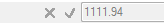
Select the cell, and then enter the text or numbers needed; your entries automatically display in the worksheet Formula bar. When you click the green check mark on the Formula bar, the value displays in the cell.
Keep in mind the following:
• Most constant values are treated as text and default to the General format. However, some combinations of numeric and non-numeric characters are interpreted as a particular number format. For example, an entry of 07/19/2013 automatically changes the format to the month/day/year date format. (See “Formatting Worksheet Cells” on page 1326.)
• Text is left-aligned unless the cell is formatted differently on the Alignment tab in the Format Cells dialog box (select Format > Cells from the Worksheet menu).
• Numbers entered in cells default to the General format. To change them to another format (for example, dimension or fractional), select Format > Cells from the Worksheet menu, and select the new format on the Number tab in the Format Cells dialog box.
~~~~~~~~~~~~~~~~~~~~~~~~~
Use formulas to evaluate and perform operations on drawing data. Formulas always begin with an equal sign (=) and consist of a combination of functions, cell references, or operators that combine values to produce a new value.
Formulas must be entered with a specific syntax. If the formula is not entered correctly, the formula entry itself displays in the cell, instead of the result of the formula. Two common mistakes in syntax include forgetting to use pairs of parentheses, and omitting required commas when no argument is present. Formula syntax is described in the following table.
|
Symbol |
Explanation |
Example |
|---|---|---|---|
General Syntax |
Equal sign = |
Begins each formula; also indicates a value for a variable |
=CriteriaVolume(t=wall) |
Parentheses ( ) |
Encloses a function argument; also used in arithmetic equations |
=acos(0.6) =A6+(A6*.07) |
|
Square brackets [ ] |
Encloses a record destination |
=R IN ['myformat'] |
|
Period . |
Separates a record identifier and a field identifier |
=Furniture.Type |
|
Colon : |
Separates path name levels in cell references |
=MyWorksheet:A1 |
|
Comma or semicolon , or ; |
Separates multiple values in a function argument; use a semicolon when commas are used as decimal separators by the operating system |
=sum(A2,E3) =sum(A2;E3) |
|
Single quote ' |
Encloses a string constant |
=Appliances.'Model #' |
|
Dollar sign $ |
Designates an absolute reference |
=A4*$B$1 |
|
Double period .. |
Designates a range of cells |
=sum(A10..A12) |
|
Arithmetic Operators |
Plus sign + |
Addition |
=A6+A8 |
Hyphen - |
Subtraction |
=A6-A8 |
|
Asterisk * |
Multiplication |
=A6*.06 |
|
Forward slash / |
Division |
=B3/12 |
|
Caret ^ |
Exponentiation |
=13^2 |
|
DIV |
Integer division (returns the integer quotient of the division operation) |
j:= 36 DIV 5; |
|
MOD |
Remainder division (returns the remainder of the division operation as an integer) |
k:= 36 MOD 5; |
|
Comparison Operators (used with IF function) |
Equal sign = |
Equal |
=if((L='L2'),Area,0) |
Less than and greater than signs (or Option+ = on Mac) <> or
|
Not equal |
=if((S<>'Dryer'),B9,0) |
|
Less than sign < |
Less than |
=if((C7<100),100,C7) |
|
Less than and equal signs (or Option+ < on Mac) <= or
|
Less than or equal to |
=if((E2<=G2),0.05,G2) |
|
Greater than sign > |
Greater than |
=if((C7>100),100,C7) |
|
Greater than and equal signs (or Option+ > on Mac) >= or
|
Greater than or equal to |
=if((E2>=G2),0.05,G2) |
To force the program to treat a number as text, enclose the number in single quotation marks, as in '40'; or format the cell as Text on the Number tab of the Format Cells dialog box.
Formulas follow standard algebraic rules of hierarchy. In the following example, the value in cell C28 is first multiplied by 12, and then 4.5 is subtracted from that value. The result is then divided by 12.
=((C28*12)-4.5)/12
There are several built-in functions that can be used in formulas, including mathematical functions and functions that pull information from objects in the drawing. To use one or more worksheet functions in a formula, either enter the function manually, or use the Insert > Function and Insert > Criteria commands to select a function and selection criteria (if required) from dialog boxes. See “Worksheet Functions” on page 1340 for more information about how to use functions.
If there is a logic problem or calculation error with a formula, an error code displays in the cell.
Error Code |
Explanation |
|---|---|
#NAME? |
The field name in a database header row definition does not exist in the file; see “Retrieving Record Information in a Worksheet” on page 1338 |
#VALUE! |
The argument is the wrong type of data for the formula; for example, a cell referenced in a mathematical formula contains text |
#CVAL? |
A cyclical reference cannot be resolved |
?Result? |
The result value type is unrecognized |
#OPCODE? |
Internal error |
#DIV 0! |
Division by zero error encountered |
#FAC? |
Unrecognized entry |
#OBJ! |
The worksheet name in an external reference does not exist, or the record name does not exist |
#CSTATUS? |
Functions are nested too deeply (more than ten levels deep) |
To manually enter a formula:
1. Select the cell.
2. Enter an equal sign (=), and then enter the formula. The entries automatically display in the worksheet Formula bar. A formula can consist of functions, operators, cell references, and constant values.
3. When the formula is complete, click the green check mark or press Enter to validate the entry. To cancel an entry, click the red X or press Esc.
4. The formula executes as soon as the cell entry has been validated (Auto-recalc must be selected in the worksheet preferences; see “Preferences” on page 1321).
To enter a formula with the Function and Criteria commands:
1. Select the cell.
2. Enter an equal sign (=). The entry automatically displays in the worksheet Formula bar.
3. Select Insert > Function from the Worksheet menu.
The Select Function dialog box opens.
4. Select a function from the list and click OK.
The formula is placed in the worksheet Formula bar and the cursor is placed between the parentheses, awaiting an argument, if necessary.
5. Do one of the following:
• If the function requires numbers or text, enter the argument between the parentheses and proceed to step 8.
• If the function requires selection criteria, select Insert > Criteria from the Worksheet menu.
6. If an object is selected when the Criteria command is selected, the Paste Attributes dialog box opens. Otherwise, proceed to step 7.
Do one of the following:
• To use attributes of the selected object as the only selection criteria, select the attributes and click OK. Proceed to step 8.
• To specify other criteria, or to use attributes of other objects in the drawing, click the Custom button.
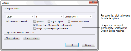
7. The Criteria dialog box opens. Set each of the three fields to the desired selection criteria. Click More Choices to specify additional criteria. Click Fewer Choices to remove added criteria. Click OK to add the criteria to the function argument.
8. When the formula is complete, click the green check mark or press Enter to validate the entry. To cancel the entry, click the red X or press Esc.
9. The formula executes as soon as the cell entry has been validated (Auto-recalc must be selected in the worksheet preferences; see “Preferences” on page 1321).
~~~~~~~~~~~~~~~~~~~~~~~~~
A formula can reference the contents of one or more other cells. The cells can be referenced within the current worksheet (internal references), or from another worksheet (external references) within the same file.
External references must include the full path name to the other worksheet. The following table shows the syntax for entering an external reference into a formula.
Syntax |
Example |
|---|---|
worksheet name:cell address |
=MyWorksheet:A1 |
worksheet name:range of addresses |
=SUM(MyWorksheet:A1..A12) |
If the name of the worksheet contains spaces, the name must be enclosed with single quotes as in the following example: ='Appliance Schedule':A1
To update an external reference, select File > Recalculate from the Worksheet menu.
Cell references in a worksheet can be either relative and absolute. When the formula that contains the reference is moved, an absolute reference always refers to the original cell address, while a relative reference changes depending on the location of the cell that contains the reference.
Use the dollar sign ($) character to indicate an absolute reference. The $ character locks the part of the cell reference it precedes, as described in the following table.
Combination |
Description |
|---|---|
$A1 |
Locks the specified column reference but leaves the row reference relative; the same column is always referred to, but the row changes if the formula is placed in a different row |
$A$1 |
Locks both the specified column and row references; regardless of where the formula is copied, it always refers to the original cell |
A$1 |
Locks the specified row reference but leaves the column reference relative; the same row is always referred to, but the column changes if the formula is placed in a different column |
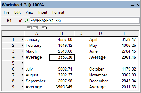
In the following example worksheet, the formula =AVERAGE(B1..B3) is in cell B4. If the formula were copied to cell E9, the formula would automatically be changed to =AVERAGE(E6..E8). Because the references are relative, both the column and row would change relative to the cell where the formula is placed—always indicating the three cells directly above the formula.
~~~~~~~~~~~~~~~~~~~~~~~~~
Database rows display data fields, calculations, or images associated with the objects in a drawing. The database header row is identified by a diamond shape next to the row number. When you create the database row, set the criteria to determine which objects will be listed in the related sub-rows. For example, you might set a header row to list all symbols in the drawing. A sub-row would then be generated for each symbol in the drawing. (If no object meets the header row criteria, no sub-rows are created.)
Many criteria combinations can be specified, such as class, object type, record information, or line weight. For example, create a list of all the rooms in a resort, or list only the green wing-backed chairs from all the two-room suites that are scattered throughout the resort.
In each column in the database header row, specify which information about the objects to display. A column can list a specific attribute of each sub-row object, such as its class or layer. A column can also list a data field contained in a record attached to each object. Or, a column can contain a constant, an image, or a formula, just as a spreadsheet cell can.
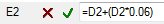
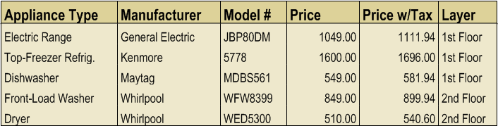
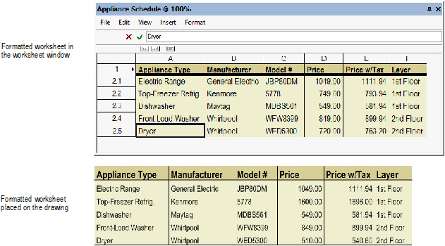
In the following example, database header row 2 has its criteria set to list all the objects in the drawing that have the appliance record attached to them. Columns A through D list the contents of the data fields in the appliance record: the appliance type, manufacturer, model number, and price. Column E contains a formula, which uses the value in column D to calculate the price of the appliance with sales tax. Column F lists which layer of the drawing contains the object.
To create a database row:
1. Right-click (Windows) or Ctrl-click (Mac) on the number of the row to change.
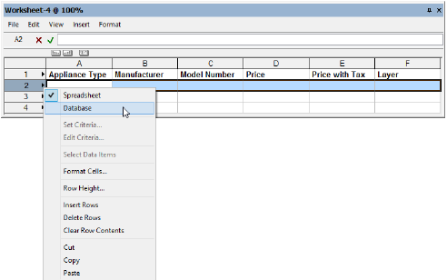
2. From the Worksheet row menu, select Database.
The Criteria dialog box opens.
3. Specify the selection criteria for which objects to display in the sub-rows. The number of objects that meet the criteria displays, to help you verify that the criteria is correct. To specify additional criteria, click More Choices.
4. Click OK to enable database functionality for the row. Beneath the header row, sub-rows are created for each drawing object that meets the criteria specified. The columns are empty until you define which data from the objects to display in each column.
5. Select each database header cell, and specify the information to be shown in each column of the row:
• To list attributes of each object (such as layer or class), see “Retrieving Object Attributes in a Worksheet” on page 1337.
• To list record data associated with each object (such as color or price), see “Retrieving Record Information in a Worksheet” on page 1338.
• To show the results of a formula for each object, see “Entering Formulas in Worksheet Cells” on page 1331.
• To show an image for each object, select Insert > Image Function from the Worksheet menu. Alternatively, select Insert Image Function from the context menu. See “Inserting Images in Worksheets” on page 1339.
6. Each sub-row cell displays the information requested. Each cell in the header row displays the total number of objects found, or, if the column returns numerical data, the header cell displays the sum for all sub-rows. Information found in each column can be sorted using the ascending, descending, and summarize buttons; see “Database Row Sort and Summary Functions” on page 1325.
To undefine a database row:
1. Right-click (Windows) or Ctrl-click (Mac) on the number of the database header row to change.
2. Select Spreadsheet.
Undefining a database row removes the database row criteria and all sub-rows. Any formulas that were defined in the columns of the header row remain intact.
A drawing object can have several attributes, such as the layer it is on, the type of object it is, the symbol name (if it is a symbol), and whether it is currently selected. You can display this information in the database rows of a worksheet.
To retrieve object information in the database rows:
1. Click the cell in the database header row where the formula will be entered.
2. Enter an equal sign (=), and then enter the criteria to display. For example, enter =C to display the name of the class to which each object belongs. The entries display in the worksheet Formula bar.
Code |
Criteria Name |
Code |
Criteria Name |
|---|---|---|---|
ALL |
Every object |
PB |
Pen background |
AR |
Arrowhead |
PF |
Pen Foreground |
ASZ |
Marker size |
PON |
Plug-in object name |
C |
Class name |
PP |
Pen pattern |
FB |
Fill background |
R |
Object record |
FF |
Fill foreground |
S |
Symbol name |
FOT |
Font |
SEL* |
Selection status |
FP |
Fill pattern |
SLST |
Slab style |
FSZ |
Font size |
SST |
Sketch style |
GFI |
Gradient fill |
ST |
Object subtype |
HFI |
Hatch fill |
T |
Object type |
IFC_ENTITY |
IFC entity |
TFI |
Tile fill |
IFI |
Image fill |
TX |
Texture |
L |
Layer name |
V |
Visibility |
LT |
Line type |
VSEL* |
Visible selection status |
LW |
Line weight |
WST |
Wall style |
N |
Object name |
|
|
* When used with the COUNT function, the SEL criterion counts objects that are actually non-selectable, such as the individual items within a group. The VSEL criterion counts only the visibly selected items, which is the same counting method used for the Object Info palette. For example, if you select and count a group that has 11 items in it, the SEL criterion returns a value of 12 (the group, plus the 11 items). The VSEL criterion returns a value of 1 (the group only). |
|||
3. Click the green check mark to validate the entry.
Database records are created in the Record Formats dialog box. These records are then assigned to objects through the Data tab of the Object Info palette. See “Visualizando e Editando Registro de Objetos” on page 261 for more information. This information can be displayed in the database rows of a worksheet.
To retrieve record information in a database row:
1. Click the cell in the database header row where the formula will be entered.
2. Enter an equal sign (=), and then enter the record information to display. The entries display in the worksheet Formula bar. The syntax for retrieving record information is:
Syntax |
Example |
|---|---|
=record name.field name |
=Furniture.Type |
A period (.) must separate the two names, or the formula will not be executed.
If the name of the record format or field name contains spaces, the name must be enclosed with single quotes as in the following example: =‘Appliance Record’.‘Model Number’
3. Click the green check mark to validate the entry.
The database information attached to each object displays in the sub-rows.
You can use the database rows in a worksheet to select the object(s) in the drawing that are related to that row. If Vectorworks Design Series is installed, you can also edit the information associated with many database objects from the worksheet.
To select database objects:
1. Either all database objects or a single database object can be selected.
• To select all database objects that meet the database row criteria, right-click (Windows) or Ctrl-click (Mac) the row number of the database header row to open the context menu.
• To select an individual database object, right-click (Windows) or Ctrl-click (Mac) the row number of the sub-row that contains the object to open the context menu.
2. From the context menu, select either Select Data Items or Select Item.
All database objects that are represented by the header row, or the individual row object, are selected. If an individual object was selected with Select Item, the drawing view changes to display the selected object. The Select Item command is unavailable if the sub-row is summarized (see “Database Row Sort and Summary Functions” on page 1325).
 To edit database objects:
In database sub-rows, some information can be edited, but some cannot. For example, the results of a calculation cannot be edited. However, if Vectorworks Design Series is installed, the data associated with a database object can be edited in the worksheet, and the object’s data record will be updated as well. For details, see “Editing Cell Contents” on page 1317.
~~~~~~~~~~~~~~~~~~~~~~~~~
 Inserting
Images in Worksheets
Inserting
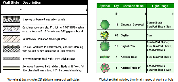
Images in WorksheetsIf Vectorworks Design Series is installed, images can be added to worksheets to provide graphic views of the objects in a drawing. The images can be either thumbnail versions of objects, or samples of the 2D attributes of objects. For example, you might create a window schedule that shows top and front thumbnail views of each type of window in your drawing, in addition to data about each window.
Worksheets can have two types of rows: spreadsheet and database. The cells in a spreadsheet row contain constants (text or numbers), or formulas. Database rows consist of a header row and sub-rows, and they show data that are associated with specific drawing objects. Images can be inserted in either type of row.
To insert an image in a cell, use the image function, which works the same as other standard worksheet functions; see “Entering Formulas in Worksheet Cells” on page 1331.
Like other functions, you can enter an image function manually on the Formula bar, or use commands and dialog boxes to build a formula that uses the image function.
A cell that uses the image function in a formula can include either a text expression or an image, but not both.
To manually enter an image formula:
1. Select the cell.
2. Enter the image function (=IMAGE). The entry automatically displays in the worksheet Formula bar. If the cell is in a database header row, no further entry is required.
3. If the cell is in a spreadsheet row, enter the rest of the formula to specify which object to display. For example, to display an image of the symbol called K-02221, enter this:
=IMAGE(S='K-02221')
4. When the formula is complete, click the green check mark to validate the entry. To cancel an entry, click the red X.
5. The formula executes, and the image(s) display (Auto-recalc must be selected in the worksheet preferences).
6. Customize the image display as described in “Entering Data in Spreadsheet Cells” on page 1329.
To enter a formula with the Image Function and Criteria commands:
1. Select the cell.
2. Select Insert > Image Function from the Worksheet menu.
The image function is placed in the worksheet Formula bar and the cursor is placed between the parentheses, awaiting an argument. If the cell is in a database header row, no further entry is required.
3. If the cell is in a spreadsheet row, enter criteria to specify which drawing object to display. Select Insert > Criteria from the Worksheet menu.
4. If an object is selected when the Criteria command is selected, the Paste Attributes dialog box opens. Otherwise, proceed to step 5.
Do one of the following:
• To use attributes of the selected object as the only selection criteria, select the attributes and click OK. Proceed to step 5.
• To specify other criteria, or to use attributes of other objects in the drawing, click Custom.
5. The Criteria dialog box opens. For each set of criteria, select the choices that apply. Click More Choices to specify additional criteria sets. Click Fewer Choices to remove added criteria sets. Click OK to add the criteria to the function argument.
6. When the formula is complete, click the green check mark to validate the entry. To cancel the entry, click the red X.
7. The formula executes, and the image(s) display (Auto-recalc must be selected in the worksheet preferences).
8. Customize the image display as described in “Entering Data in Spreadsheet Cells” on page 1329.
Click here for a video tip about this topic (Internet access required).
Worksheet functions take an argument, perform an action, and return a value or values. There are two basic types of functions: those that use the value(s) you enter, and those that use information from objects in the drawing. The arguments required by the two function types are different.
• Number or text arguments: Functions that begin with a lower case letter typically require a number value or a cell address as the argument. For example, the acos function returns the arccosine of the value that is specified in the function argument. The argument you enter can be a mathematical expression (such as 3/5), an address of a cell that contains a number (such as A12), or an actual number. The argument for all trigonometry functions must be in radians.
• Criteria arguments: Functions that begin with a capital letter must be applied to one or more specific objects in the drawing. In a cell in a database header row, a function is automatically applied to the object listed in each sub-row, so no criteria argument is required.
However, in a spreadsheet cell, you must enter criteria to select the objects the function applies to. For example, the Area function returns the combined area of all 2D objects that meet the criteria. To specify which objects to obtain the area of, either use the Insert > Criteria command on the Worksheet menu, or enter the criteria manually. For details about how to specify criteria such as the object type, class, or visibility, see the developer oriented documentation here:
http://developer.vectorworks.net/index.php/VS:Search_Criteria#Search_Criteria_Tables
http://developer.vectorworks.net/index.php/VS:Function_Reference_Appendix#attrCrit
The following table lists all of the worksheet functions available, as well as what kind of argument the function takes.
You may want to display an attribute associated with a drawing object in the worksheet (such as the object’s class, or which layer it is on); see “Retrieving Object Attributes in a Worksheet” on page 1337.
Function (argument) |
Description |
Example |
Related Functions |
|---|---|---|---|
acos(number) |
The arccosine of a number. The arccosine is the angle whose cosine is number. The returned angle is given in radians in the range 0 to pi. Number is the cosine of the angle, and must be from -1 to 1. |
=acos(3/5) (returns the angle for which the cosine value is 3/5) |
cos |
Angle(criteria) |
The angle (measured from horizontal) of the objects that meet the specified criteria, in degrees. Use this function to return the angles of lines and walls (measured from horizontal), the span angles of arcs, and the slope angles of slabs. |
Database header cell: =Angle (returns the angle of each object in the database) Spreadsheet cell: =Angle((t=arc)&(n='arc-1')) (returns the sweep angle of the arc object named “arc-1” in the drawing) |
|
Area(criteria) |
The total area of 2D objects that meet the specified criteria, based on the Area units in the Units dialog box |
Database header cell: =Area (returns the area of each object in the database) Spreadsheet cell: =Area(t=rect) (returns the combined area of all rectangle objects in the drawing) |
Perim |
asin(number) |
The arcsine of a number. The arcsine is the angle whose sine is number. The returned angle is given in radians in the range -pi/2 to pi/2. To express the arcsine in degrees, use the rad2deg function (or multiply the result by 180/pi). Number is the sine of the angle and must be from -1 to 1. |
=asin(A3) (returns the angle for which the sine value is given in cell A3) |
sin |
atan(number) |
The arctangent of a number. The arctangent is the angle whose tangent is number. The returned angle is given in radians in the range -pi/2 to pi/2. To express the arctangent in degrees, use the rad2deg function (or multiply the result by 180/pi). Number is the tangent of the angle in question. |
=atan(4/3) (returns the angle for which the tangent value is 4/3) |
tan |
average(number1, number2...) |
The average (mean) of the arguments |
=average(85,70,95) (returns the average of the three numbers) |
max, min, sum |
BotBound(criteria) |
The bottom 2D boundary (minimum y coordinate) of the objects that meet the specified criteria |
Database header cell: =BotBound (returns the bottom 2D boundary of each object in the database) Spreadsheet cell: =BotBound(t=locus) (returns the bottom 2D boundary of the locus that has the lowest bottom 2D boundary value in the drawing) |
LeftBound, RightBound, TopBound |
ComponentArea |
The area of one side of the specified wall or slab component, minus any holes. Index is the 1-based index identifying the component. |
Database header cell: =ComponentArea(2) (returns the area of the second component for each wall or slab object in the database) Spreadsheet cell: =ComponentArea(t=wall,1) (returns the combined area of the first components for all walls in the drawing) |
ComponentVolume, ComponentName |
ComponentName |
The name of the specified wall or slab component. Index is the 1-based index identifying the component. |
Database header cell: =ComponentName(2) (returns the name of the second component for each wall or slab object in the database) Spreadsheet cell: =ComponentName(t=wall,1) (returns the name of the first component for all walls in the drawing) |
ComponentVolume, ComponentArea |
ComponentVolume |
The volume of the specified component, minus any holes. Index is the 1-based index identifying the component. |
Database header cell: =ComponentVolume(2) (returns the volume of the second component for each wall or slab object in the database) Spreadsheet cell: =ComponentVolume(t=wall,1) (returns the combined volume of the first components for all walls in the drawing) |
ComponentArea, ComponentName |
concat(text1, text2, text3) |
Joins several text strings into one text string |
=concat(B3,', ',B4) (returns the contents of cells B3 and B4 as a single string, separated by a comma and a space) |
|
cos(number) |
The cosine of a given angle. Number is the angle in radians for which the cosine is calculated. |
=cos(deg2rad(23)) (converts a 23-degree angle to its radian equivalent, and returns the cosine of the angle) |
acos |
Count(criteria) |
The number of objects that meet the specified criteria |
Database header cell: =Count (returns the total number of objects for each row in the database) Spreadsheet cell: =Count(s='simple sofa') (returns the total number of symbol objects named “simple sofa” in the drawing) |
|
CurtWallFrameLength(criteria, class) |
The combined length of the curtain wall frames that meet the specified criteria and are in the specified class. To find all frames in a curtain wall, use an empty class name. |
Database header cell: =CurtWallFrameLength('') (returns the combined length of the curtain wall frames for each curtain wall in the database) Spreadsheet cell: =CurtWallFrameLength(t=wall, '') (returns the combined length of the curtain wall frames for all curtain walls in the drawing) |
CurtWallPnlAreaNet, CurtWallPnlAreaGross |
CurtWallPnlAreaGross(criteria, class) |
The combined gross area of the curtain wall panels in the walls that meet the specified criteria and are in the specified class. The gross area includes portions of the panel covered by frames. To find all panels in a curtain wall, use an empty class name. |
Database header cell: =CurtWallPnlAreaGross('') (returns the combined gross area of the curtain wall panels for each curtain wall in the database) Spreadsheet cell: =CurtWallPnlAreaGross(t=wall, '') (returns the combined gross area of the curtain wall panels for all curtain walls in the drawing) |
CurtWallFrameLength, CurtWallPnlAreaNet |
CurtWallPnlAreaNet (criteria, class) |
The net area of the curtain wall panels in the walls that meet the specified criteria and are in the specified class. The net area includes only the visible area bounded by frames. To find all panels in a curtain wall, use an empty class name. |
Database header cell: =CurtWallPnlAreaNet ('Class-1') (returns the combined net area of the curtain wall panels assigned to the class “Class-1” for each curtain wall in the database) Spreadsheet cell: =CurtWallPnlAreaNet(t=wall, 'Class-1') (returns the combined net area of the curtain wall panels assigned to the class “Class-1” for all curtain walls in the drawing) |
CurtWallFrameLength, CurtWallPnlAreaGross |
deg2rad(number) |
Converts a number from degrees to radians. Number is the value in degrees to be converted to radians. |
=deg2rad(47) (converts the 47-degree angle measurement to its radian equivalent) |
|
exp(number) |
e raised to the power of number. The constant e equals 2.71828182845904, the base of the natural logarithm. Number is the exponent applied to the base e. |
=exp(2) (returns the numeric value of e raised to the power of 2) |
ln |
GetIfcProperty (Vectorworks Architect/Landmark required) |
The value of a specific IFC property associated with an IFC object. The criteria is a string with two elements separated by a period. The first element is either an IFC entity or PSet name, and the second element is the name of the IFC property. |
=GETIFCPROPERTY ('ifcfurnishingelement.name') (returns the Name value for IFC objects whose IFC entity is IfcFurnishingElement) |
|
Height(criteria) |
The combined delta y (height) of objects that meet the specified criteria |
Database header cell: =Height (returns the height (delta y) for each object in the database) Spreadsheet cell: =Height(sel=true) (returns the combined height (delta y) value of the selected objects in the drawing) |
Width |
if ((logical_test), value_if_true, value_if_false) |
Use value_if_true if logical_test is true, value_is_false if logical_test is false. Use this function to conduct conditional tests on values and formulas and to branch based on the results of that test. The outcome of the test determines the value returned by the If function. The logical_test can be any value or expression that can be evaluated to true or false. Up to seven If statements can be nested as value_if_true, value_if_false arguments. Boolean statements within an if statement must be in parentheses. Text within an if statement should be enclosed within quotation marks. |
=if((C7>100),100,C7) when commas are used as decimal separators by the operating system, use semicolons instead: =if((C7>100);100;C7) (if the value in cell C7 is greater than 100, the value in this cell is 100; otherwise, the value in this cell is the same as the value in cell C7) |
|
Image(criteria) (Vectorworks Design Series required) |
The image associated with the object that meets the specified criteria. In the cell format, specify whether to show a thumbnail of the object, or the 2D attributes applied to the object. |
Database header cell: =Image (returns the image for each object in the database) Spreadsheet cell: =Image(s='cabinet') (returns the image of the symbol named “Cabinet”) |
|
int(number) |
Removes any fractional part of a number. Number is the real number to be changed to an integer. |
=int(B9) (returns the value in cell B9 without its fractional component) |
round |
IsFlipped(criteria) |
The flipped state of the objects that meet the specified criteria |
Database header cell: =IsFlipped (returns the flip state for each object in the database) Spreadsheet cell: =IsFlipped(PON=window) (returns the total number of window objects in the drawing that are flipped) |
|
LeftBound(criteria) |
The left side 2D boundary (minimum x coordinate) of the objects that meet the specified criteria |
Database header cell: =LeftBound (returns the left 2D boundary for each object in the database) Spreadsheet cell: =LeftBound(t=locus) (returns the left 2D boundary of the leftmost locus in the drawing) |
BotBound, TopBound, RightBound |
Length(criteria) |
The length of lines, walls, or path-based objects that meet the specified criteria |
Database header cell: =Length (returns the length for each object in the database) Spreadsheet cell: =Length(t=line) (returns the total length of all line objects in the drawing) |
|
ln(number) |
The natural logarithm (base e). Number is the positive real number for which the logarithm is calculated. |
=ln(12) (returns the natural logarithm of 12) |
exp |
log(number) |
The base 10 logarithm. Number is the positive real number for which the logarithm is calculated. |
=log(2) (returns the base 10 logarithm of 2) |
ln |
max(number1, number2,...) |
The largest number in the list of arguments. Number is 1 – 14 numbers for which the maximum value is to be found. |
=max(C5,C7,C9) (returns the largest of the numbers that are in cells C5, C7, and C9) |
min |
min(number1, number2,...) |
The smallest number in the list of arguments. Number is 1 – 14 numbers for which the minimum value is to be found. |
=min(C5,C7,C9) (returns the smallest of the numbers that are in cells C5, C7, and C9) |
max |
ObjectType(criteria) |
The numeric object type ID of objects that meet the specified criteria For a list of object type IDs, see the developer oriented documentation here: http://developer.vectorworks.net/index.php/VS:Function_Reference_Appendix#objects |
Database header cell: =ObjectType (returns the object type value for each object in the database) Spreadsheet cell: =ObjectType(sel=true) (returns the object type value of the selected object; for example, the object type value for a light is 81) |
|
Perim(criteria) |
The combined perimeter of objects that meet the specified criteria |
Database header cell: =Perim (returns the perimeter for each object in the database) Spreadsheet cell: =Perim(sel=true) (returns the total perimeter of all selected objects) |
|
rad2deg(number) |
Converts a number from radians to degrees. Number is the value in radians to be converted to degrees. |
=rad2deg(0.5235987) (converts the radian angle measurement to its degree equivalent) |
|
RightBound(criteria) |
The right side 2D boundary (maximum x coordinate) of the objects that meet the specified criteria |
Database header cell: =RightBound (returns the right 2D boundary for each object in the database) Spreadsheet cell: =RightBound(t=rect) (returns the right 2D boundary of the rightmost rectangle in the drawing) |
BotBound, TopBound, LeftBound |
RoofArea_Heated |
The heated area of the roof (minus the eve overhang) along the slope, combined for all objects that meet the specified criteria |
Database header cell: =RoofArea_Heated (returns the heated area for each roof and roof face object in the database) Spreadsheet cell: =RoofArea_Heated (st=roofface) (returns the combined heated area of all roof face objects in the drawing) |
RoofArea_HeatedProj |
RoofArea_HeatedProj |
The heated area of the roof (minus the eve overhang) projected to the layer plane, combined for all objects that meet the specified criteria |
Database header cell: =RoofArea_HeatedProj (returns the heated area for each roof and roof face object in the database, as projected to the layer plane) Spreadsheet cell: =RoofArea_Heatedproj(t=roof) (returns the combined heated area of all roof objects in the drawing, as projected to the layer plane) |
RoofArea_Heated |
RoofArea_Total |
The total area of the roof along the slope |
Database header cell: =RoofArea_Total (returns the total area for each roof and roof face object in the database) Spreadsheet cell: =RoofArea_Total(st=roofface) (returns the combined total area of all roof face objects in the drawing) |
RoofArea_TotalProj |
RoofArea_TotalProj |
The total area of the roof, projected to the layer plane |
Database header cell: =RoofArea_TotalProj (returns the total area for each roof and roof face object in the database, as projected to the layer plane) Spreadsheet cell: =RoofArea_Totalproj(t=roof) (returns the combined total area of all roof objects in the drawing, as projected to the layer plane) |
RoofArea_Total |
round(number) |
Rounds the specified number to the nearest whole number |
=round(D11) (returns the value in cell D11 rounded to the nearest whole number) |
int |
sin(number) |
The sine of a given angle. Number is the angle in radians for which the sine is calculated. |
=sin(deg2rad(32)) (converts a 32-degree angle to its radian equivalent, and returns the sine of the angle) |
asin |
SlabStyleName (Vectorworks Architect required) |
The name of a slab style |
Database header cell: =SlabStyleName (returns the name of the slab style for each slab object in the database) |
|
SlabThickness (Vectorworks Architect required) |
The combined thickness of slab objects (floors and roof faces) that meet the specified criteria |
Database header cell: =SlabThickness (returns the thickness for each object in the database) Spreadsheet cell: =SlabThickness(PON=slab) (returns the combined thickness of all slab objects in the drawing) |
|
sqrt(number) |
A positive square root. Number is the number for which the square root is calculated. |
=sqrt(D27) (returns the square root of the number in cell D27) |
|
Substring(text/function, delimiter, index) |
Splits a single string into an array of strings using a delimiter, and outputs each string at the specified index |
=SUBSTRING(('kitchen;bedroom;bathroom;basement', ';', 2) (returns “bedroom,” which is the second substring in the specified string) |
|
sum(number1, number2,...) |
The sum of all numbers in the list of arguments. Number is 1 – 14 numbers for which the sum is calculated. |
=sum(A2,A10..A12) (returns the sum of the numbers contained in cells A2, A10, A11, and A12) |
Average |
SurfaceArea(criteria) |
The total surface area of all objects that meet the criteria, based on the Area units in the Units dialog box |
Database header cell: =SurfaceArea (returns the surface area for each object in the database) Spreadsheet cell: =SurfaceArea(st=sphere) (returns the total surface area of all sphere objects in the drawing) |
|
tan(number) |
The tangent of the given angle. Number is the angle in radians for which the tangent is calculated. |
=tan(deg2rad(32)) (converts a 32-degree angle to its radian equivalent, and returns the tangent of the angle) |
atan |
TopBound(criteria) |
The top 2D boundary (maximum y coordinate) of the objects that meet the specified criteria |
Database header cell: =TopBound (returns the top 2D boundary for each object in the database) Spreadsheet cell: =TopBound(sel=true) (returns the top 2D boundary of the topmost selected object) |
BotBound, LeftBound, RightBound |
value(text) |
Converts a text string that represents a number to a number |
=value('2e3') (returns the numeric value of 2 times 10 raised to the power of 3) |
|
Volume(criteria) |
The total volume of all objects that meet the criteria, based on the Volume units in the Units dialog box. |
Database header cell: =Volume (returns the volume for each object in the database) Spreadsheet cell: =Volume(t=xtrd) (returns the total volume of all extrude objects in the drawing) |
|
WallArea_Gross |
The combined 2D gross surface area of one wall face for walls that meet the specified criteria |
Database header cell: =WallArea_Gross (returns the gross surface area of one wall face for each wall object in the database) Spreadsheet cell: =WallArea_Gross(t=wall) (returns the combined gross surface area of one wall face for all walls in the drawing) |
WallArea_Net |
WallArea_Net |
The combined 2D net surface area of one wall face, without door, window, and inserted symbol areas, for walls that meet the specified criteria |
Database header cell: =WallArea_Net (returns the net surface area of one wall face, minus inserted object areas, for each object in the database) Spreadsheet cell: =WallArea_Net(t=wall) (returns the combined net surface area of one wall face, minus inserted object areas, for all walls in the drawing) |
WallArea_Gross |
WallAverageHeight |
The average height of a wall, including wall peaks and different starting and ending heights |
Database header cell: =WallAverageHeight (returns the average height for each wall object in the database) Spreadsheet cell: =WallAverageHeight((t=wall)& (returns the average height of all walls that are selected in the drawing) |
|
WallStyleName (Vectorworks Architect/Landmark required) |
The name of a wall style |
Database header cell: =WallStyleName (returns the name of the wall style for each wall object in the database) |
|
WallThickness |
The combined thickness of wall objects that meet the specified criteria |
Database header cell: =WallThickness (returns the thickness for each wall object in the database) Spreadsheet cell: =WallThickness(t=wall) (returns the combined thickness of all walls in the drawing) |
|
Width(criteria) |
The combined delta x (width) of objects that meet the specified criteria |
Database header cell: =Width (returns the width (delta x) for each object in the database) Spreadsheet cell: =Width(sel=true) (returns the combined width (delta x value) of the selected object) |
Height |
XCenter(criteria) |
The x coordinate of the center point of an object that meets the specified criteria |
Database header cell: =XCenter (returns the x coordinate value of the center of the 2D boundary for each object in the database) Spreadsheet cell: =XCenter(sel=true) (returns the x coordinate value of the center of the 2D boundary of the selected object) |
YCenter, ZCenter, XCoordinate |
XCoordinate(critiera) |
The x coordinate of the insertion point for symbols, point plug-in objects, and loci. The returned value is relative to the user origin. |
Database header cell: =XCoordinate (returns the x coordinate value for each object in the database) |
YCoordinate, ZCoordinate, XCenter |
YCenter(criteria) |
The y coordinate of the center point of an object that meets the specified criteria |
Database header cell: =YCenter (returns the y coordinate value of the center of the 2D boundary for each object in the database) Spreadsheet cell: =YCenter(sel=true) (returns the y coordinate value of the center of the 2D boundary of the selected object) |
XCenter, ZCenter, YCoordinate |
YCoordinate(criteria) |
The y coordinate of the insertion point for symbols, point plug-in objects, and loci. The returned value is relative to the user origin. |
Database header cell: =YCoordinate (returns the y coordinate value for each object in the database) |
XCoordinate, ZCoordinate, YCenter |
ZCenter(criteria) |
The z coordinate of the center point of an object that meets the specified criteria |
Database header cell: =ZCenter (returns the z coordinate value of the center of the 3D boundary for each object in the database) Spreadsheet cell: =ZCenter(sel=true) (returns the z coordinate value of the center of the 3D boundary of the selected object) |
XCenter, YCenter, ZCoordinate |
ZCoordinate(criteria) |
The z coordinate of the insertion point for symbols, point plug-in objects, and loci. The returned value is relative to the user origin. |
Database header cell: =ZCoordinate (returns the z coordinate value for each object in the database) |
XCoordinate, YCoordinate, ZCenter |
~~~~~~~~~~~~~~~~~~~~~~~~~
Data from a wide variety of worksheet formats can be imported into a file, including worksheet data from other programs and worksheets from other Vectorworks files.
To import a worksheet into the current file, a blank worksheet must exist in the active drawing as a destination for the imported worksheet. During import, the spreadsheet data is imported, but the formulas (logic) are not.
To import worksheet data into a Vectorworks file:
1. From the Resource Browser, select Resources > New Resource > Worksheet.
The Create Worksheet dialog box opens.
2. Specify the same number of rows and columns that are present in the worksheet to be imported.
3. Select File > Import > Import Worksheet.
4. Select the worksheet file to be imported. The worksheet must be in one of the following formats:
• Tab delimited text (.txt)
• Comma delimited text (.csv)
• DIF (.dif)
• SYLK (.slk)
5. Click Open. The worksheet is imported into the open worksheet in the Vectorworks file.
To import a Vectorworks worksheet from another Vectorworks file:
1. From the Resource Browser, locate the file containing the worksheet using the Resources > Find command, or from a Favorites file. See “Accessing Existing Resources” on page 225 for more information.
2. Select the worksheet to import, and click Import. (Alternatively, drag the worksheet resource into the desired Vectorworks file to insert it as a drawing object; see “Worksheets as Graphic Objects” on page 1356.)
The selected worksheet is imported into the current file.
The following procedure is an example of how to import a table from Microsoft Word into a Vectorworks worksheet.
To import a Word table into a worksheet:
1. In Word, select the entire table to be imported.
2. In versions of Word prior to 2007, select Table > Convert > Table to Text. In Word 2007 and later, select the Table Tools > Layout > Convert to Text.
The Convert Table to Text dialog box opens.
3. In the dialog box, click Tabs for the separation identifier.
4. Click OK.
5. Save the table.
If the file consists of only the table, select File > Save As. In the Save As dialog box that opens, select Text Only from the Save as type list, and click OK.
If the table is part of a larger file, copy the table to the Clipboard. Select File > New, and paste the table text into the new document. Save the file as a text file.
6. Return to the Vectorworks file and import the table as described in “Importing Worksheet Data from Another Program” on page 1355.
Vectorworks worksheet files can be exported and read by spreadsheet programs, such as Excel, as well as by some word processing programs. Because many of these programs have different format requirements, several export formats are available. These include comma delimited, tab delimited, merge, DIF, and SYLK. Using the tab delimited format, for example, creates a file that can be opened as a table in Microsoft Word.
To export a worksheet from a Vectorworks file:
1. Open the worksheet to export.
2. Select File > Export > Export Worksheet.
3. The Export Worksheet dialog box opens.
Select the format for the export, and whether to export all rows or only the selected rows. Click OK and specify the name and location of the exported worksheet.
4. Click Save. The specified worksheet rows are exported to the desired location in the set format.
A worksheet can be included in a drawing as a graphic object. The worksheet object can be moved to any location on the drawing, but it cannot be resized. Use the Attributes palette to modify the fill, pen, and line thickness attributes of the entire worksheet object. To edit the contents of the worksheet, open it from the Resource Browser, or from the drawing itself.
To include a worksheet as an object on a drawing:
1. From the Resource Browser, select the desired worksheet.
The worksheet must be a part of the current drawing. If the worksheet is part of another drawing, first import it into the current drawing. Select the worksheet from the Resource Browser and then select Resources > Import. (See “Importing Worksheet Data from Another Program” on page 1355.)
2. Select Resources > Worksheet On Drawing.
The worksheet is now included in the drawing as a graphic object. It can be moved like any other graphic object and placed where desired. If the worksheet is currently open, the contents of the worksheet in the drawing are replaced with an X.
Alternatively, double-click the worksheet in the Resource Browser to place it in the drawing file, or select the worksheet in the Resource Browser and drag it to the desired location in the drawing file. Both methods automatically select Worksheet on Drawing and place the worksheet as a graphic object. If you use the drag and drop method, the top left corner of the worksheet is placed at the point where the mouse is released in the drawing file.
To edit a worksheet included as a drawing object:
1. From the Resource Browser, select the desired worksheet.
2. Select Resources > Open.
Alternatively, double-click the worksheet object in the drawing.
3. The worksheet is opened and available for editing. The contents of the worksheet in the drawing are replaced with an X. Close the worksheet to display the worksheet contents in the drawing.
This simple tutorial explains how to create a customized schedule that links wall objects in a drawing to a database worksheet. The schedule will display data for wall areas, wall thicknesses, labor cost, material cost, taxes, and total cost per wall style quantity.
The WorksheetTutorial.vwx file contains the data required to perform the tutorial steps. Though wall styles are a Vectorworks Design Series feature, any Vectorworks license can use the wall styles that already exist in the tutorial file. Download the file here (Internet connection required) and open it in Vectorworks to begin.
There are three ways to create a schedule using worksheets. This tutorial uses the first option below.
• Start with a blank worksheet, and create the schedule from scratch. See “Creating a Blank Worksheet” on page 1313.
• Create a schedule based on a common record format of a set of objects (wall data, in this example). This option allows you to select the criteria you wish to display from all the available object criteria. See “Creating Reports” on page 1312.
• Start with a preformatted schedule and customize it to achieve your goals. See “Creating Schedules” on page 1858.
To create a blank worksheet:
1. From the Resources menu in the Resource Browser, select New Resource > Worksheet. The Create Worksheet dialog box opens.
2. Enter “Wall Area and Costs” as the name for the new worksheet, and click OK. You will add more rows and columns later.
A blank worksheet window opens.
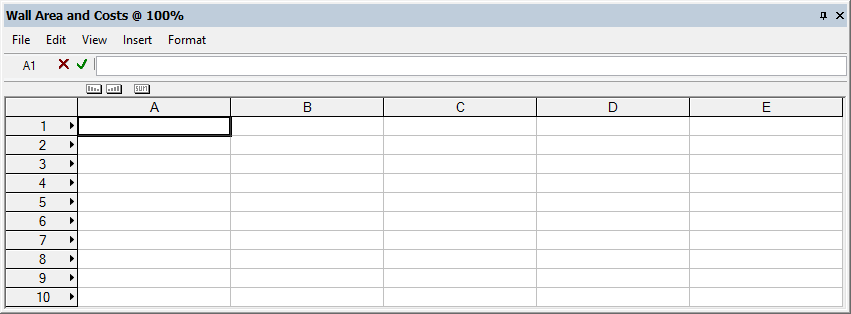
Next, create a database of the objects in the drawing from which to extract the wall area data. You can combine multiple criteria to collect the desired subset of objects.
For this tutorial, a single database of wall objects will be created and limited to a specified set of wall styles.
An alternative would be to create one database per wall style and include multiple databases in the same worksheet. However, for very large databases, it is recommended to create separate worksheets rather than include multiple databases into a single worksheet.
To set the database criteria:
1. Right-click (Windows) or Ctrl-click (Mac) on the header box for row 3.
2. From the Row context menu, select Database. The Criteria dialog box opens.
3. Set the three criteria options as follows:
• Type
• is
• Wall
4. Click More Choices, and set the next three criteria as follows:
• Wall Style
• is
• Aspen Interior Walls
5. Click More Choices, and set the next three criteria as follows:
• Wall Style
• is
• Ext-CIP Conc 36”-Footing
To include all wall styles in the schedule, do not enter criteria for walls and wall styles; instead, use the following criteria: Record, Wall Data, is present.
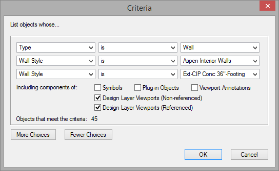
6. Click OK to set the criteria. The database of walls for the specified set of wall styles is created. The database header (row 3) now has a diamond next to the row number. Beneath row 3 are sub-rows for each object in the database (3.1 through 3.45).
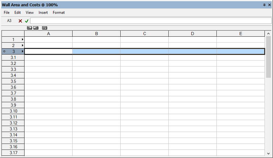
For this tutorial, you need to expand the worksheet. Since no data has been assigned to the columns yet, it does not matter where the columns are added.
Use one of the following methods to add three columns to the worksheet, for a total of eight.
• Select Insert > Columns. An empty column is added to the left of the current column.
• Right-click (Windows) or Ctrl-click (Mac) the column header where you want to add a column, and select Insert Columns from the context menu.
• Position the cursor at the bottom right corner of the worksheet to activate a special resize cursor; drag as needed to add columns to the right side of the worksheet.
Next, add database functions to the worksheet to extract the desired data from the database. Enter formulas for each column in the database header row cells. The database header row can be hidden before the worksheet is placed on the drawing.
For this tutorial, the following data will be extracted:
• Wall Style Name
• Gross Wall Area
• Net Wall Area
• Wall Thickness
To extract the data associated with the walls in the database:
1. Click the following cells and enter the formula shown to extract data for each item in the database. Be sure to include the equal sign (=) before each item.
• In A3 enter =WALLSTYLENAME
• In B3 enter =WALLAREA_GROSS
• In C3 enter =WALLAREA_NET
• In D3 enter =WALLTHICKNESS
Alternatively, use the worksheet menu command Insert > Function to insert functions.
2. By default, numerical data is unformatted and must be formatted to display appropriate units. Formatting applied to database header row cells is automatically applied to all sub-rows for that column.
Right-click (Windows) or Ctrl-click (Mac) each of the following cells, and select Format Cells from the context menu. The Format Cells dialog box opens. On the Number tab, select the format option shown and click OK.
• For B3 select Dimension Area
• For C3 select Dimension Area
• For D3 select Dimension
Alternatively, use the worksheet menu command Format > Cells to format cells.
3. Add labels for columns A through D by typing names in the cells in row 2.
• In A2 enter Wall Style Name
• In B2 enter Wall Area (Gross)
• In C2 enter Wall Area (Net)
• In D2 enter Wall Thickness
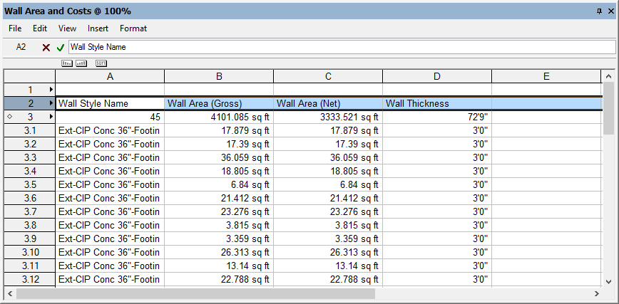
Various types of data can be extracted from Vectorworks objects into a worksheet database, as described in the following topics.
• “Worksheet Functions” on page 1340
• “Retrieving Object Attributes in a Worksheet” on page 1337
• “Retrieving Record Information in a Worksheet” on page 1338
• “Entering Formulas in Worksheet Cells” on page 1331
Instead of listing each wall individually in the database, you can summarize all walls with the same wall style, automatically calculating the total quantities for each, and shortening the list.
To summarize the wall styles:
1. Click on the header box for row 3 to select it. Three icons display just below the Formula bar.
2. Click and drag the Summarize icon to the header box for column A, which contains wall styles.
3. The number of sub-rows is reduced to only two (one row per wall style). The numerical values in columns B, C, and D are now sums. While this is desired for the wall area gross and net columns, you probably want to show the thickness value as the thickness of an individual wall, rather than all walls combined. To do so, apply another Summarize icon to column D.
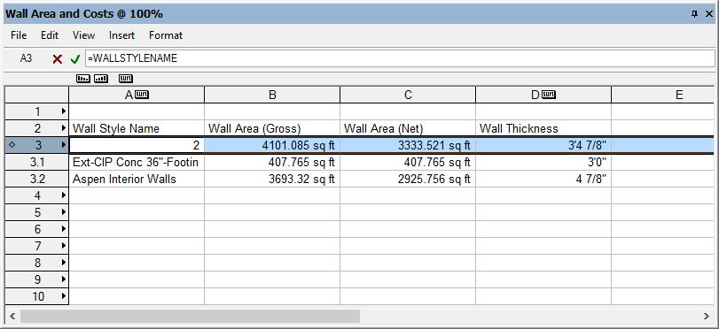
Next, calculate costs using worksheet operations and formulas.
For this tutorial, the following data will be calculated:
• Labor cost per wall style
• Material cost per wall style
• Taxes
• Total cost
To calculate costs with formulas:
1. Add labels for columns E through H by typing names in the cells in row 2.
• In E2 enter Labor Cost
• In F2 enter Material Cost
• In G2 enter Taxes
• In H2 enter Total Cost
2. Click the following cells and enter the formula shown to determine the cost sums. Be sure to include the equal sign (=) before each item.
• In E3 enter =C3*15.5 (multiply the value in C3 by 15.5, the estimated rate of labor cost per area unit)
• In F3 enter =C3*9.2 (multiply the value in C3 by 9.2, the estimated material cost per area unit)
• In G3 enter =F3*.08 (multiply the value in F3 by 0.08, the estimated tax rate)
• In H3 enter =E3+F3+G3 (calculate the total cost of labor, material, and taxes)
Instead of entering the tax rate directly into the calculation, an alternative and more flexible approach is to set the tax rate in a separate spreadsheet cell and simply reference it in the calculation.
3. Format all of the cost data the same way. Select the four cost header cells (E3 through H3), and then right-click (Windows) or Ctrl-click (Mac) and select Format Cells from the context menu. The Format Cells dialog box opens. On the Number tab, select the options shown and click OK.
• Select Decimal
• In Dec. Places, enter 2
• Select Use Commas
• In Leader, enter $ (dollar sign)
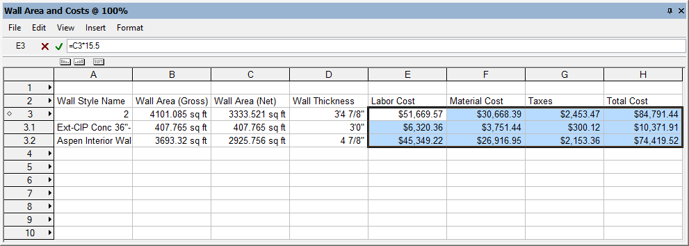
Next, set up totals at the bottom of the columns as appropriate. The cells in the database header row (in this case, row 3) display sums for all of the database columns. Reference these database header row cells in spreadsheet cells to set up the totals.
To set up the totals:
1. Click the following cells and enter the formula shown to show sums from the database header row. Be sure to include the equal sign (=) before each item.
• In B4 enter =B3
• In C4 enter =C3
• In E4 enter =E3
• In F4 enter =F3
• In G4 enter =G3
• In H4 enter =H3
2. Select cells B4 and C4, right-click (Windows) or Ctrl-click (Mac), and select Format Cells from the context menu. On the Number tab, select Dimension Area and click OK.
3. Select cells E4 through H4, right-click (Windows) or Ctrl-click (Mac), and select Format Cells from the context menu. On the Number tab, select the options shown and click OK.
• Select Decimal
• In Dec. Places, enter 2
• Select Use Commas
• In Leader, enter $ (dollar sign)
4. Click cell A1 and enter Wall Areas and Costs as the schedule title.
5. Select row 2, right-click (Windows) or Ctrl-click (Mac), and select Insert Rows from the context menu to add an empty row between the schedule title and the column labels.
6. Select the empty rows at the bottom of the worksheet (6 through 11), right-click (Windows) or Ctrl-click (Mac), and select Delete Rows from the context menu.
7. Select View > Database Headers and then View > Grid Lines to hide the database header row and grid lines in the table.
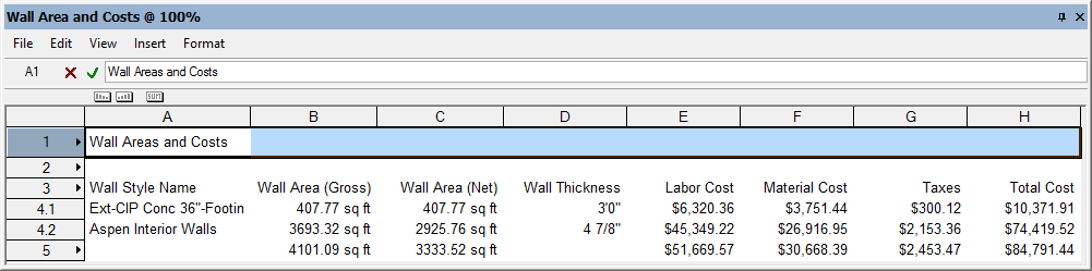
Finally, select cells and use the Format Cells command to format the worksheet as needed. You can change the font, font style, size, and color to format the text. Add cell borders, and change cell background color, as desired. Change the text alignment in cells, and resize rows and columns, if necessary.
See “Formatting Worksheet Cells” on page 1326 for details.