Utilities

The Engineering Properties command automatically calculates the engineering properties of a 2D object.

The Engineering Properties dialog box opens. The data that displays is selection-dependent.

• Plane properties (area, perimeter, and absolute coordinates of the centroid of the object)

• Moments of inertia, section modulus’, and radii of gyration about the object’s centroidal axes

For a single closed surface and a locus point, the moments of inertia and radii of gyration about the axes that pass through the locus are also displayed, as well as the horizontal and vertical distances from the locus to the centroid of the object.

Parameter	Description
Units	Update the displayed information to reflect the selected unit of measurement
Place locus at centroid	Select to add a locus at the centroid of the selected object after closing the Engineering Properties dialog box
Place properties on drawing	Select to place a list of the properties at the next mouse click after closing the Engineering Properties dialog box
Write properties to a file	Select to send the properties to a text file; specify the file name and location after closing the Engineering Properties dialog box

Obtaining Volumetric Properties

The volumetric properties of a 3D object can be obtained with the Volumetric Properties command.

The Volumetric Properties dialog box opens, displaying the surface area, volume, and center of mass of the object.

Parameter	Description
Place locus at center of mass	Places a 3D locus at the center of mass of the object
Place properties on drawing	Places the volumetric properties as text on the drawing at a specified location

3. Set the parameters and click OK. If Place locus at center of mass was selected, the 3D locus is placed automatically on the object. If Place properties on drawing was selected, click in the drawing file to specify the location of the text.

Compressing Images

The bitmap images and image resources in a Vectorworks file can be compressed with the JPEG compression method, to save file space. JPEG compression can significantly reduce bitmap image file size, but can result in the loss of fine detail for some images.

The compression method and file size for a selected image display in the Object Info palette. Images that are already compressed by the JPEG compression method remain unchanged.

A selected bitmap file displays “Bitmap” as the object type at the top of the Object Info palette. A bitmap file may already have had PNG compression applied at import; the Compress Images command changes its compression format to JPEG.

Compressing Selected Bitmap Images

3. Select Apply JPEG Compression to Selected Bitmap Objects. Click OK to compress the selected images.

Compressing All Bitmap Images and/or Image Resources

The JPEG compression method can be applied to all bitmap images in the file. For the best possible reduction in file size, images that have been imported as resources (shown as image resources in the Resource Browser) can also be compressed by the JPEG compression method.

2. Select Apply JPEG Compression to All. Choose whether to apply the JPEG compression to all bitmap images in the drawing, image resources, or both. Click OK to compress the images.

Tracing Bitmaps

The Trace Bitmap command traces bitmap objects and picture objects (images which have been imported with the Import PICT as Picture command). It creates a group of vector lines from the image.

Parameter	Description
Maximum width in pixels	Specify the maximum number of pixels to be recognized as a single line; pixel counts above the selected value are traced
Collinearity Sensitivity	Select a value to define the segment size and accuracy of the trace

The time it takes to trace the image can vary from seconds to hours. The tracing time required is determined by the image size, as well as the line threshold and collinearity sensitivity settings selected.

Creating 3D Objects from 2D Objects

The Create 3D Object from 2D command places a 3D version of a 2D object in a drawing. The command applies to the following 2D objects with 3D counterparts.

* The spur gear, worm gear, sprocket, and pulley convert to a 3D object and 3D hub object.

This command creates the 3D equivalent of a selected 2D object. If a 2D object with no 3D equivalent is selected, a beep sounds, a notice indicates that the object cannot be converted, and the object is deselected.

Spring Calculator

The Spring Calculator command solves for spring rates and unit stresses based on compression spring parameters.

Parameter	Description
Units	Sets the spring dimension units to Inches, cm, or mm
Method	Select the method; as data is entered, the other dimensions are automatically calculated
Dimensions	The fields available depend upon the Method and the Type of Ends selected
Outside Diameter	Enter the outside diameter
Mean Diameter	Enter the mean diameter
Wire Diameter	Enter the wire diameter
Solid Height	Enter the solid height
No. of Active Coils	Enter the number of active coils
Type of Ends	Select Closed and Ground, Open and Ground, Closed, or Open to set the type of ends on the spring
Properties	The properties of the spring can be selected from the list or manually entered
Material	Select the material to be used for the spring or select <Other> to set the Modulus of Elasticity manually
Mod. of Elasticity	Automatically entered based on the material selected; displayed in pounds per square inch, newtons per square centimeter, or newtons per square millimeter, depending on selected units. If <Other> was selected, enter the Modulus of Elasticity manually.
Spring Rate	Automatically calculated based on the spring parameters; displayed in the selected units
Unit Stress	Automatically calculated based on the spring parameters; displayed in the selected units
Place 2D spring on drawing	Select to draw a 2D spring according to the above parameters; if both check boxes are selected, the 2D and 3D springs are automatically aligned in the drawing
Place 3D spring on drawing	Select to draw a 3D spring according to the above parameters; if both check boxes are selected, the 2D and 3D springs are automatically aligned in the drawing

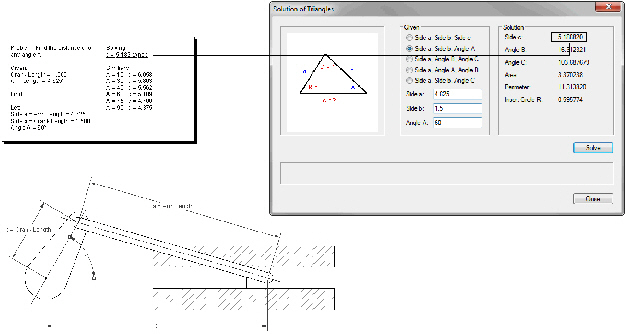
Belt Length Calculator

The Belt Length Calculator solves for either belt length or center distance between two pulleys.

Parameter	Description
Find	Select whether to calculate the Belt Length or the Center Distance between pulleys
(1) Diameter	Enter the first pitch diameter
(2) Diameter	Enter the second pitch diameter
(3) Center Distance	If calculating the belt length, enter the Center Distance
Belt Length	If calculating the center distance, enter the Belt Length
Place data on drawing	Select to insert the calculated data on the drawing

If the center distance value is unknown, leave the field blank, and then click Solve. The minimum distance is displayed. Click Solve again to solve for the belt length based on the minimum center distance.

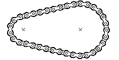
Chain Length Calculator

The Chain Length calculator solves for either the length of a chain or center distance between two sprockets.

Parameter	Description
Chain and Sprocket Data
Find	Select whether to calculate the Chain Length or the Center Distance between sprockets
Std.Chain No. (Pitch)	Select the pitch of the chain
(1) Number of Teeth, Sprocket #1	Enter the number of teeth of sprocket #1
(2) Number of Teeth, Sprocket #2	Enter the number of teeth of sprocket #2
(3) Center Distance or Chain Length	If calculating the chain length, enter the Center Distance; if calculating the center distance, enter the Chain Length
Chain Length or Center Distance	Depending on the Find selected, the chain length or center distance calculation is displayed
Placement Options
Place chain on drawing	Inserts the continuous chain onto the drawing, based on the specified and calculated values
Place sprockets on drawing	Inserts the two sprockets onto the drawing based on the specified and calculated value
Group the objects	Select to group the objects when inserted onto the drawing; if deselected, the objects are ungrouped when inserted onto the drawing and are editable in the Object Info palette
Place data on drawing	When selected, inserts the calculated data onto the drawing

The Chain Length value can be entered based on the number of pitches multiplied by the pitch value.

If the center distance value is unknown, leave the field blank, and then click Solve. The minimum distance is displayed. Click Solve again to solve for the chain length based on the minimum center distance.

5. If placement options were selected, the cursor changes to a bull’s eye. Click in the drawing to insert the chain and/or sprockets. If Place data on the drawing was selected, click again to insert the calculated data.

Control Values for Keys

The Control Values for Keys calculator solves for the key depths of a given shaft and the key size.

2. Enter the shaft diameter size. Select Recommended Key Size to use the recommended key size according to the ASME or ISO standard; otherwise, select Custom Key Size to enter custom key sizes.

Parameter	Description
Nom. Shaft Diameter (D)	Enter the size of the shaft
Recommended Key Size	Select to use the recommended key size according to the ASME or ISO standard
Square	Select to use the recommended square key
Rectangular	Select to use the recommended rectangular key
Key Width (W)/Height (H)	Displays the dimensions of the recommended key
Custom Key Size	Select to use custom key sizes
Key Width (W)	Enter the width of the key
Key Height (H)	Enter the height of the key
Solution
Depth to Bottom of Key (S)	Displays the dimension from the bottom of the shaft to the bottom of the key
Depth to Top of Key (T)	Displays the dimension from the bottom of the shaft to the top of the key
Place data on drawing	Select to insert the calculated data on the drawing

Shaft Analysis

The Shaft Analysis utility analyzes the results of a twisting moment being applied to a round solid or hollow shaft.

Parameter	Description
Shaft Analysis	Enter the shaft properties; the analysis results are based on the properties provided
(1) Outside Diameter	Enter the outside diameter of the shaft; select the desired units from the list
Inside Diameter	Enter the inside diameter of the shaft; enter zero for a solid shaft
Polar Moment of Inertia	Automatically calculated from the outside and inside diameters
(2) Length	Enter the length of the shaft
Shear Modulus	Enter the value of the shear modulus; select the desired units from the list
Solutions	Select and enter the known value
(3) Twisting Moment	Enter the twisting moment; select the desired units from the list
Maximum Shear Stress	Enter the maximum shear stress; the units are set by the Shear Modulus value
(4) Angle of Twist	Enter the angle of twist in degrees

The unknown values in the Solutions section are solved based on the information given.

Centroid

The Centroid utility calculates the centroid, or center of gravity, of a 2D shape. The utility shows the location of the centroid and can place a locus at that point. For more information, see “Obtaining Engineering Properties” on page 1813.

3. The location of the centroid is displayed. Select Place locus at centroid to place a locus marker at the centroid of the object.

If the object is moved, the locus point does not remain centroidal unless the object and locus point are grouped and then moved.

Conversion Factors

2. In the Multiply field, enter the number of units to convert. Select the original unit of measure from the Multiply list.

3. Select the target unit of measure from the To Obtain list. The conversion results display in the To Obtain field and the conversion factor displays in the By field.

Solution of Triangles

2. Select the format of the known values, and then enter them in the fields below.

3D Properties

The 3D Properties utility calculates a 3D object’s center of mass, radii of gyration, and mass properties based on density or specific gravity, surface area, and volume. This can be used for 3D objects such as a sweep, extrude, or solid.

The 3D Properties dialog box displays the object surface area, volume, radii of gyration, and center of mass.

Parameter	Description
Units	Select the unit for displaying values
Places locus at centroid	Select to place a locus point at the 3D center of the object
Place properties on drawing	Select to place a grouped text block containing the 3D property values on the drawing at the next mouse click
Write properties to a file	Select to create a text file containing the 3D property values

The Mass Properties dialog box displays the weight, mass, and mass moments of inertia of the object.

Parameter	Description
Input
System of Units	Select the units to use for the calculation
Property to Use	Select whether to display properties based on the density or specific gravity
Value	Enter the material density or gravity value

Simple Beam Analysis

The Simple Beam Analysis command opens a message box displaying the calculated values that correspond to the cursor position.

A message dialog box opens at the bottom of the screen, displaying x (location on the beam), vx (shear), mx (bending moment), sx (shearing stress), and y (deflection) values.

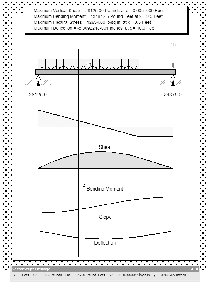
The values displayed depend on the location of the cursor along the beam and the Calculation Interval specified in the Beam Properties dialog box.

3. Click on a blank area of the drawing to stop the analysis. Close the message dialog box.

To lock the values in the message dialog box, click on a point along the beam. The values at this point can then be studied or written down for future analysis. Select the Simple Beam Analysis command again to continue checking values along the beam.

Simple Beam Calculator

The Simple Beam Calculator command provides a quick way to analyze a simply-supported beam with a single load.

2. Select the desired configuration, and then enter the values to be calculated.

Parameter	Description
Configuration	Select the simple beam configuration to analyze; the preview window updates to correspond to the selected configuration
Input
Units	Select Imperial or Metric (SI) as the displayed unit value
Beam and Load Data	Select Imperial or Metric (SI) as the displayed unit value
Beam Length (L)	Enter the length of the beam
Concentrated Load (P)	Enter the value of a concentrated load or loads
Dist. from end of beam (a)	Enter the distance from the end of the beam to the load
Distributed Load (w)	Enter the value per unit length of a distributed load
Beam Properties
Modulus of Elasticity	Enter the modulus of elasticity of the beam
Moment of Inertia	Enter the moment of inertia of the beam
Section Modulus	Enter the section modulus of the beam
Select Structural Shape and Materials	Opens the Select Structural Shape and Material dialog box for selection of a structural shape, series, size, and material for the beam and axis about which the properties are needed (see “Structural Shapes and Details” on page 439). Click OK to return to the Simple Beam Calculator dialog box; the beam properties section is updated with these values for the selected structural shape, and the fields can be manually adjusted as needed.
Solution
Reaction at Left End (rL)	Displays the reaction at the left support
Reaction at Right End (rR)	Displays the reaction at the right support
Moment at Left End (mL)	Displays the bending moment at the left support
Moment at Right End (mR)	Displays the bending moment at the right support
Max. Shear (vMax)	Displays the maximum vertical shear
Max. Bending Moment (mMax)	Displays the maximum bending moment
Max. Shear Stress	Displays the maximum shear stress
Max. Deflection	Displays the maximum deflection
at x (from left end)	Displays the point from the left end of the beam at which the maximum deflection occurs

Acorn nut (Inch)	Lock washer (Inch, Metric, DIN, ISO)	Spur gear *
Angle (AISC Inch and Metric, BSI, JIS, ANZ, DIN)	Needle bearing	Spur gear rack
Ball bearing	Nut (Inch, Metric, DIN, ISO)	Square tubing (AISC Inch and Metric, BSI, JIS, ANZ, DIN)
Bearing lock nut	Parallel pin (DIN)	Swing bolt
Bevel gears	Pillow block bearing	Swing eye bolt
Bulb flat (BSI, JIS, DIN)	Plain washer (Inch, Metric, DIN, ISO)	Taper pin (Inch, DIN)
Carriage bolt (Inch, Metric)	Pulley *	Tapered roller bearing
Channel (AISC Inch and Metric, JIS, ANZ, DIN)	Rectangular tubing (AISC Inch and Metric, BSI, JIS, ANZ, DIN)	T-bolt
Clevis pin (Inch, Metric, DIN, ISO	Retaining ring (Inch, DIN)	Tee (AISC Inch and Metric, BSI, JIS, DIN)
Compression spring - 1 and 2	Retaining washer (DIN)	Thrust bearing
Conical compression spring	Rivet - large (Inch)	Thumb screw (Inch)
Cotter pin (Inch)	Rivet - small (Inch)	Torsion spring - Front, End
Die spring	Rivet (DIN)	Tubular rivet (DIN)
Dowel pin (Inch)	Roller bearing	U-bolt
Extension spring - Front, End	Roller chain - circular	Wide flange (AISC Inch and Metric, BSI, JIS, ANZ, DIN)
Eye bolt	Roller chain - linear	Wing nut (DIN)
Flanged bearing - 2 and 4 hole	Roller chain - offset link	Wing nut type A, B, C, D (Inch)
Hole - drilled	Round tubing (AISC Inch and Metric, BSI, JIS, ANZ, DIN)	Woodruff key
Hole - tapped (Inch, Metric)	Screw and nut (Inch, Metric, DIN, ISO)	Wood screw
I-Beam (AISC Inch and Metric, BSI, JIS, ANZ, DIN)	Set screw (Inch, Metric, DIN, ISO)	Worm
J-Bolt (Inch, Metric)	Shaft	Worm gear *
Key	Sheet metal screw (Inch, Metric)	Z-Section
Knurled thumb nut (Inch, DIN)	Shoulder screw (Inch, Metric, DIN, ISO)
Lag screw (Inch, Metric)	Sprocket *